Polygons#
In addition to points, lines, areas, rasters, and trimeshes, Datashader can quickly render large collections of polygons (filled polylines). Datashader’s polygon support depends on data structures provided by the spatialpandas library. SpatialPandas extends Pandas and Parquet to support efficient storage and manipulation of “ragged” (variable length) data like polygons. Instructions for installing spatialpandas are given at the bottom of this page.
SpatialPandas Data Structures#
Pandas supports custom column types using an “ExtensionArray” interface. SpatialPandas provides two Pandas ExtensionArrays that support polygons:
spatialpandas.geometry.PolygonArray: Each row in the column is a singlePolygoninstance. As with shapely and geopandas, each Polygon may contain zero or more holes.spatialpandas.geometry.MultiPolygonArray: Each row in the column is aMultiPolygoninstance, each of which can store one or more polygons, with each polygon containing zero or more holes.
Datashader assumes that the vertices of the outer filled polygon will be listed as x1, y1, x2, y2, etc. in counter-clockwise (CCW) order around the polygon edge, while the holes will be in clockwise (CW) order. All polygons (both filled and holes) must be “closed”, with the first vertex of each polygon repeated as the last vertex.
        graph TD;
    subgraph SP[ ]
        A[Polygon]:::spatialpandas -->|used in| E[PolygonArray]:::spatialpandas
        B[MultiPolygon]:::spatialpandas -->|used in| F[MultiPolygonArray]:::spatialpandas
        E -->|used in| G[GeoDataFrame or<div></div> GeoSeries]:::spatialpandas
        spatialpandas(SpatialPandas):::spatialpandas_title
        F -->|used in| G
    end

    subgraph SH[ ]
        shapely(Shapely):::shapely_title
        H[Polygon]:::shapely -->|converts to| A
        I[MultiPolygon]:::shapely -->|converts to| B
    end

    subgraph GP[ ]
        geopandas(GeoPandas):::geopandas_title
        J[GeoDataFrame or<div></div> GeoSeries]:::geopandas
    end

    subgraph PD[ ]
        pandas(Pandas):::pandas_title
        K[DataFrame or<div></div> Series]:::pandas
    end

    subgraph SPD[ ]
        spatialpandas.dask(SpatialPandas.Dask):::dask_title
        L[DaskGeoDataFrame or<div></div> DaskGeoSeries]:::dask
    end

    M(Datashader):::datashader_title

    F -->|usable in| K
    E -->|usable in| K

    G -->|converts to| L

    G <-->|converts to| J

    G -->|usable by| M
    L -->|usable by| M
    J -->|usable by| M
    K -->|usable by| M

    classDef spatialpandas fill:#4e79a7,stroke:#000,stroke-width:0px,color:black;
    classDef shapely fill:#f28e2b,stroke:#000,stroke-width:0px,color:black;
    classDef geopandas fill:#59a14f,stroke:#000,stroke-width:0px,color:black;
    classDef dask fill:#76b7b2,stroke:#000,stroke-width:0px,color:black;
    classDef datashader fill:#b07aa1,stroke:#000,stroke-width:0px,color:black;
    classDef pandas fill:#edc948,stroke:#000,stroke-width:0px,color:black;
    classDef spatialpandas_title fill:#fff,stroke:#4e79a7,stroke-width:7px,color:black,fill-opacity:.9,font-weight: bold;
    classDef shapely_title fill:#fff,stroke:#f28e2b,stroke-width:7px,color:black,fill-opacity:.9,font-weight: bold;
    classDef geopandas_title fill:#fff,stroke:#59a14f,stroke-width:7px,color:black,fill-opacity:.9,font-weight: bold;
    classDef dask_title fill:#fff,stroke:#76b7b2,stroke-width:7px,color:black,fill-opacity:.9,font-weight: bold;
    classDef pandas_title fill:#fff,stroke:#edc948,stroke-width:7px,color:black,fill-opacity:.9,font-weight: bold;
    classDef datashader_title fill:#fff,stroke:#b07aa1,stroke-width:7px,color:black,fill-opacity:.9,font-weight: bold;
    classDef subgraph_style fill:#fff;

    style SP fill:grey,stroke:#fff,stroke-width:0px
    style SH fill:grey,stroke:#fff,stroke-width:0px
    style GP fill:grey,stroke:#fff,stroke-width:0px
    style PD fill:grey,stroke:#fff,stroke-width:0px
    style SPD fill:grey,stroke:#fff,stroke-width:0px
Importing Required Libraries#
import pandas as pd
import numpy as np
import dask.dataframe as dd
import colorcet as cc
import datashader as ds
import datashader.transfer_functions as tf
import spatialpandas as sp
import spatialpandas.geometry
import spatialpandas.dask
Simple Example#
Here is a simple example of a two-element MultiPolygonArray. The first element specifies two filled polygons, the first with two holes. The second element contains one filled polygon with one hole.
polygons = sp.geometry.MultiPolygonArray([
    # First Element
    [[[0, 0, 1, 0, 2, 2, -1, 4, 0, 0],         # Filled quadrilateral (CCW order)
      [0.5, 1,  1, 2,  1.5, 1.5,  0.5, 1],     # Triangular hole (CW order)
      [0, 2, 0, 2.5, 0.5, 2.5, 0.5, 2, 0, 2]], # Rectangular hole (CW order)

     [[-0.5, 3, 1.5, 3, 1.5, 4, -0.5, 3]],],   # Filled triangle

    # Second Element
    [[[1.25, 0, 1.25, 2, 4, 2, 4, 0, 1.25, 0],          # Filled rectangle (CCW order)
      [1.5, 0.25, 3.75, 0.25, 3.75, 1.75, 1.5, 1.75, 1.5, 0.25]],]]) # Rectangular hole (CW order)
The filled quadrilateral starts at (x,y) (0,0) and goes to (1,0), then (2,2), then (-1,4), and back to (0,0); others similarly go left to right (but drawing in either CCW or CW order around the edge of the polygon depending on whether they are filled or holes).
Since a MultiPolygonArray is a pandas/dask extension array, it can be added as a column to a DataFrame. For convenience, you can define your DataFrame as sp.GeoDataFrame instead of pd.DataFrame, which will automatically include support for polygon columns:
df = sp.GeoDataFrame({'polygons': polygons, 'v': range(1, len(polygons)+1)})
df
| polygons | v | |
|---|---|---|
| 0 | MultiPolygon([[[0.0, 0.0, 1.0, 0.0, 2.0, 2.0, ... | 1 |
| 1 | MultiPolygon([[[1.25, 0.0, 1.25, 2.0, 4.0, 2.0... | 2 |
Rasterizing Polygons#
Polygons are rasterized to a Canvas by Datashader using the Canvas.polygons method. This method works like the existing glyph methods (.points, .line, etc), except it does not have x and y arguments. Instead, it has a single geometry argument that should be passed the name of a PolygonArray or MultiPolygonArray column in the supplied DataFrame. For comparison we’ll also show the polygon outlines rendered with Canvas.line (which also supports geometry columns):
%%time
cvs = ds.Canvas()
agg = cvs.polygons(df, geometry='polygons', agg=ds.sum('v'))
filled = tf.shade(agg)
float(agg.min()), float(agg.max())
CPU times: user 3.52 s, sys: 515 ms, total: 4.03 s
Wall time: 6.12 s
(1.0, 3.0)
%%time
cvs = ds.Canvas()
agg = cvs.line(df, geometry='polygons', agg=ds.sum('v'), line_width=4)
unfilled = tf.shade(agg)
float(agg.min()), float(agg.max())
CPU times: user 2.57 s, sys: 178 ms, total: 2.74 s
Wall time: 2.86 s
(0.0032808413085092525, 3.0)
tf.Images(filled, unfilled)
 |  |
Here as you can see each polygon is filled or outlined with the indicated value from the v column for that polygon specification. The sum aggregator for the filled polygons specifies that the rendered colors should indicate the sum of the v values of polygons that overlap that pixel, and so the first element (v=1) has an overlapping area with value 2, and the second element has a value of 2 except in overlap areas where it gets a value of 3. Each plot is normalized separately, so the filled plot uses the colormap for the range 1 (light blue) to 3 (dark blue), while the outlined plot ranges from 1 to 2.
You can use polygons from within interactive plotting programs with axes to see the underlying values by hovering, which helps for comparing Datashader’s aggregation-based approach (right) to standard polygon rendering (left):
import holoviews as hv
from holoviews.operation.datashader import rasterize
from holoviews.streams import PlotSize
PlotSize.scale=2 # Sharper plots on Retina displays
hv.extension("bokeh")

hvpolys = hv.Polygons(df, vdims=['v']).opts(color='v', tools=['hover'])
hvpolys + rasterize(hvpolys, aggregator=ds.sum('v')).opts(tools=['hover'])


Realistic Example#
Here is a more realistic example, plotting the unemployment rate of the counties in Texas. To run you need to run bokeh sampledata or install the package bokeh_sampledata.
from bokeh.sampledata.us_counties  import data as counties
from bokeh.sampledata.unemployment import data as unemployment

counties = { code: county for code, county in counties.items()
            if county["state"] in ["tx"] }

county_boundaries = [[[*zip(county["lons"] + county["lons"][:1],
                            county["lats"] + county["lats"][:1])]
                     for county in counties.values()]]

county_rates = [unemployment[county_id] for county_id in counties]

boundary_coords = [[np.concatenate(list(
    zip(county["lons"][::-1] + county["lons"][-1:],
        county["lats"][::-1] + county["lats"][-1:])
))] for county in counties.values()]

boundaries = sp.geometry.PolygonArray(boundary_coords)

county_info = sp.GeoDataFrame({'boundary': boundaries,
                               'unemployment': county_rates})
# Discard the output from one aggregation of each type, to avoid measuring Numba compilation times
tf.shade(cvs.polygons(county_info, geometry='boundary', agg=ds.mean('unemployment')));
tf.shade(cvs.line(county_info, geometry='boundary', agg=ds.any()));
tf.shade(cvs.line(county_info, geometry='boundary', agg=ds.any(), line_width=1.5));
%%time
cvs = ds.Canvas(plot_width=600, plot_height=600)
agg = cvs.polygons(county_info, geometry='boundary', agg=ds.mean('unemployment'))
filled = tf.shade(agg)
CPU times: user 30.7 ms, sys: 4.1 ms, total: 34.8 ms
Wall time: 35.3 ms
%%time
agg = cvs.line(county_info, geometry='boundary', agg=ds.any())
unfilled = tf.shade(agg)
CPU times: user 19.9 ms, sys: 3.71 ms, total: 23.6 ms
Wall time: 24.1 ms
%%time
agg = cvs.line(county_info, geometry='boundary', agg=ds.any(), line_width=3.5)
antialiased = tf.shade(agg)
CPU times: user 1.62 s, sys: 100 ms, total: 1.72 s
Wall time: 1.84 s
tf.Images(filled, unfilled, antialiased)
 |  |  |
Using GeoPandas and Converting to SpatialPandas#
You can utilize a GeoPandas GeoSeries of Polygon/MultiPolygon objects with Datashader:
import geodatasets as gds
import geopandas

geodf = geopandas.read_file(gds.get_path('geoda health'))
geodf = geodf.to_crs(epsg=4087) # simple cylindrical projection
geodf['boundary'] = geodf.geometry.boundary
geodf['centroid'] = geodf.geometry.centroid
geodf.head()
| cartodb_id | countyfp | statefp | statename | countyname | countyfips | tractname | ratio | statemhir | tractmhir | ... | AmericanI | Asianalon | NativeHaw | TwoorMor | Hispanico | Whitealon | county | geometry | boundary | centroid | |
|---|---|---|---|---|---|---|---|---|---|---|---|---|---|---|---|---|---|---|---|---|---|
| 0 | 80.0 | 057 | 12 | Florida | Hillsborough County, Florida | 12057.0 | Census Tract 108.14, Hillsborough County, Florida | 0.575 | 47212.0 | 27143.0 | ... | 0.5 | 3.9 | 0.1 | 2.5 | 26.0 | 52.3 | County | POLYGON ((-9176896.069 3102142.81, -9176672.09... | LINESTRING (-9176896.069 3102142.81, -9176672.... | POINT (-9176144.094 3102914.106) |
| 1 | 398.0 | 213 | 48 | Texas | Henderson County, Texas | 48213.0 | Census Tract 9509.01, Henderson County, Texas | 0.752 | 52576.0 | 39558.0 | ... | 0.8 | 0.6 | 0.1 | 1.6 | 11.8 | 79.4 | County | POLYGON ((-10737226.084 3601372.655, -10737024... | LINESTRING (-10737226.084 3601372.655, -107370... | POINT (-10670372.997 3585811.751) |
| 2 | 409.0 | 409 | 48 | Texas | San Patricio County, Texas | 48409.0 | Census Tract 102.01, San Patricio County, Texas | 0.708 | 52576.0 | 37231.0 | ... | 0.9 | 1.1 | 0.1 | 1.4 | 55.4 | 40.8 | County | POLYGON ((-10825232.165 3101367.699, -10825221... | LINESTRING (-10825232.165 3101367.699, -108252... | POINT (-10825227.649 3101341.923) |
| 3 | 647.0 | 005 | 24 | Maryland | Baltimore County, Maryland | 24005.0 | Census Tract 4209, Baltimore County, Maryland | 0.485 | 74149.0 | 35996.0 | ... | 0.4 | 5.7 | 0.1 | 2.3 | 4.8 | 60.5 | County | POLYGON ((-8559974.583 4389270.415, -8559908.7... | LINESTRING (-8559974.583 4389270.415, -8559908... | POINT (-8531547.508 4393047.522) |
| 4 | 712.0 | 031 | 13 | Georgia | Bulloch County, Georgia | 13031.0 | Census Tract 1104.03, Bulloch County, Georgia | 0.367 | 49342.0 | 18103.0 | ... | 0.4 | 1.6 | 0.1 | 1.6 | 3.6 | 64.6 | County | POLYGON ((-9131186.283 3624024.168, -9128365.7... | LINESTRING (-9131186.283 3624024.168, -9128365... | POINT (-9099609.103 3606395.64) |
5 rows × 67 columns
Optionally, you can convert the GeoPandas GeoDataFrame to a SpatialPandas GeoDataFrame. Since version 0.16, Datashader supports direct use of geopandas GeoDataFrames without having to convert them to spatialpandas. See GeoPandas.
%%time
sgeodf = sp.GeoDataFrame(geodf)
sgeodf.head()
CPU times: user 3.77 s, sys: 741 ms, total: 4.51 s
Wall time: 5.76 s
| cartodb_id | countyfp | statefp | statename | countyname | countyfips | tractname | ratio | statemhir | tractmhir | ... | AmericanI | Asianalon | NativeHaw | TwoorMor | Hispanico | Whitealon | county | geometry | boundary | centroid | |
|---|---|---|---|---|---|---|---|---|---|---|---|---|---|---|---|---|---|---|---|---|---|
| 0 | 80.0 | 057 | 12 | Florida | Hillsborough County, Florida | 12057.0 | Census Tract 108.14, Hillsborough County, Florida | 0.575 | 47212.0 | 27143.0 | ... | 0.5 | 3.9 | 0.1 | 2.5 | 26.0 | 52.3 | County | Polygon([[-9176896.069490857, 3102142.81028444... | Line([-9176896.069490857, 3102142.8102844423, ... | Point([-9176144.093665784, 3102914.1062057978]) |
| 1 | 398.0 | 213 | 48 | Texas | Henderson County, Texas | 48213.0 | Census Tract 9509.01, Henderson County, Texas | 0.752 | 52576.0 | 39558.0 | ... | 0.8 | 0.6 | 0.1 | 1.6 | 11.8 | 79.4 | County | Polygon([[-10737226.08366159, 3601372.65522642... | Line([-10737226.08366159, 3601372.6552264225, ... | Point([-10670372.997268908, 3585811.7511676615]) |
| 2 | 409.0 | 409 | 48 | Texas | San Patricio County, Texas | 48409.0 | Census Tract 102.01, San Patricio County, Texas | 0.708 | 52576.0 | 37231.0 | ... | 0.9 | 1.1 | 0.1 | 1.4 | 55.4 | 40.8 | County | Polygon([[-10825232.16513267, 3101367.69938376... | Line([-10825232.16513267, 3101367.69938376, -1... | Point([-10825227.6488587, 3101341.923372258]) |
| 3 | 647.0 | 005 | 24 | Maryland | Baltimore County, Maryland | 24005.0 | Census Tract 4209, Baltimore County, Maryland | 0.485 | 74149.0 | 35996.0 | ... | 0.4 | 5.7 | 0.1 | 2.3 | 4.8 | 60.5 | County | Polygon([[-8559974.583463615, 4389270.41508, -... | Line([-8559974.583463615, 4389270.41508, -8559... | Point([-8531547.50804809, 4393047.522164391]) |
| 4 | 712.0 | 031 | 13 | Georgia | Bulloch County, Georgia | 13031.0 | Census Tract 1104.03, Bulloch County, Georgia | 0.367 | 49342.0 | 18103.0 | ... | 0.4 | 1.6 | 0.1 | 1.6 | 3.6 | 64.6 | County | Polygon([[-9131186.282820305, 3624024.16785201... | Line([-9131186.282820305, 3624024.1678520194, ... | Point([-9099609.103138514, 3606395.639896559]) |
5 rows × 67 columns
Converting from SpatialPandas to GeoPandas/Shapely#
A MultiPolygonArray can be converted to a geopandas GeometryArray using the to_geopandas method.
%%time
pd.Series(sgeodf.boundary.array.to_geopandas())
CPU times: user 2.01 s, sys: 48.1 ms, total: 2.06 s
Wall time: 2.13 s
0       LINESTRING (-9176896.069 3102142.81, -9176672....
1       LINESTRING (-10737226.084 3601372.655, -107370...
2       LINESTRING (-10825232.165 3101367.699, -108252...
3       LINESTRING (-8559974.583 4389270.415, -8559908...
4       LINESTRING (-9131186.283 3624024.168, -9128365...
                              ...
3979    LINESTRING (-8981066.272 4286189.123, -8979277...
3980    LINESTRING (-10093522.353 4848294.332, -100914...
3981    LINESTRING (-11875382.161 4163749.261, -118718...
3982    LINESTRING (-12811368.351 4808827.899, -128029...
3983    LINESTRING (-10738305.326 4530365.309, -107383...
Length: 3984, dtype: geometry
Individual elements of a MultiPolygonArray can be converted into shapely shapes using the to_shapely method
sgeodf.geometry.array[3].to_shapely()

Plotting Polygons with Datashader#
Plotting as filled polygons#
Datashader can also plot polygons as filled shapes. Here’s an example using a spatialpandas GeoDataFrame.
# Discard the output to avoid measuring Numba compilation times
tf.shade(cvs.polygons(sgeodf, geometry='geometry', agg=ds.mean('cty_pop200')));
%%time
cvs = ds.Canvas(plot_width=650, plot_height=400)
agg = cvs.polygons(sgeodf, geometry='geometry', agg=ds.mean('cty_pop200'))
tf.shade(agg)
CPU times: user 331 ms, sys: 18.9 ms, total: 350 ms
Wall time: 352 ms

Plotting as centroid points#
# Discard the output to avoid measuring Numba compilation times
cvs.points(sgeodf, geometry='centroid', agg=ds.mean('cty_pop200'));
%%time
agg = cvs.points(sgeodf, geometry='centroid', agg=ds.mean('cty_pop200'))
tf.spread(tf.shade(agg), 2)
CPU times: user 2.46 s, sys: 171 ms, total: 2.63 s
Wall time: 2.72 s

Polygon Perimeter/Area calculation#
The spatialpandas library provides highly optimized versions of some of the geometric operations supported by a geopandas GeoSeries, including parallelized Numba implementations of the length and area properties:
{"MultiPolygon2dArray length":    sgeodf.geometry.array.length[:4],
 "GeoPandas length":              geodf.geometry.array.length[:4],
 "MultiPolygonArray area":        sgeodf.geometry.array.area[:4],
 "GeoPandas area":                geodf.geometry.array.area[:4],}
OMP: Info #276: omp_set_nested routine deprecated, please use omp_set_max_active_levels instead.
{'MultiPolygon2dArray length': array([6.90868437e+03, 3.40192966e+05, 9.62593429e+01, 3.32774104e+05]),
 'GeoPandas length': array([6.90868437e+03, 3.40192966e+05, 9.62593429e+01, 3.32774104e+05]),
 'MultiPolygonArray area': array([2.99167772e+06, 2.91166029e+09, 2.45110832e+02, 2.07981346e+09]),
 'GeoPandas area': array([2.99167772e+06, 2.91166029e+09, 2.45110832e+02, 2.07981346e+09])}
Speed differences:
# Duplicate 500 times
sgeodf_large = pd.concat([sgeodf.geometry] * 500)
geodf_large = pd.concat([geodf.geometry] * 500)
length_ds = %timeit -o -n 3 -r 1 geodf_large.array.length
length_gp = %timeit -o -n 3 -r 1 sgeodf_large.array.length
print("\nMultiPolygonArray.length speedup: %.2f" % (length_ds.average / length_gp.average))
1.27 s ± 0 ns per loop (mean ± std. dev. of 1 run, 3 loops each)
2min 2s ± 0 ns per loop (mean ± std. dev. of 1 run, 3 loops each)

MultiPolygonArray.length speedup: 0.01
area_ds = %timeit -o -n 3 -r 1 geodf_large.array.area
area_gp = %timeit -o -n 3 -r 1 sgeodf_large.array.area
print("\nMultiPolygonArray.area speedup: %.2f" % (area_ds.average / area_gp.average))
992 ms ± 0 ns per loop (mean ± std. dev. of 1 run, 3 loops each)
1min 22s ± 0 ns per loop (mean ± std. dev. of 1 run, 3 loops each)

MultiPolygonArray.area speedup: 0.01
Other GeoPandas operations could be sped up similarly by adding them to spatialpandas.
Parquet support#
SpatialPandas geometry arrays can be stored in Parquet files, which support efficient chunked columnar access that is particularly important when working with Dask for large files. To create such a file, use .to_parquet:
sgeodf.to_parquet('sgeodf.parq')
A parquet file containing geometry arrays should be read using the spatialpandas.io.read_parquet function:
from spatialpandas.io import read_parquet
read_parquet('sgeodf.parq').head(2)
| cartodb_id | countyfp | statefp | statename | countyname | countyfips | tractname | ratio | statemhir | tractmhir | ... | AmericanI | Asianalon | NativeHaw | TwoorMor | Hispanico | Whitealon | county | geometry | boundary | centroid | |
|---|---|---|---|---|---|---|---|---|---|---|---|---|---|---|---|---|---|---|---|---|---|
| 0 | 80.0 | 057 | 12 | Florida | Hillsborough County, Florida | 12057.0 | Census Tract 108.14, Hillsborough County, Florida | 0.575 | 47212.0 | 27143.0 | ... | 0.5 | 3.9 | 0.1 | 2.5 | 26.0 | 52.3 | County | Polygon([[-9176896.069490857, 3102142.81028444... | Line([-9176896.069490857, 3102142.8102844423, ... | Point([-9176144.093665784, 3102914.1062057978]) |
| 1 | 398.0 | 213 | 48 | Texas | Henderson County, Texas | 48213.0 | Census Tract 9509.01, Henderson County, Texas | 0.752 | 52576.0 | 39558.0 | ... | 0.8 | 0.6 | 0.1 | 1.6 | 11.8 | 79.4 | County | Polygon([[-10737226.08366159, 3601372.65522642... | Line([-10737226.08366159, 3601372.6552264225, ... | Point([-10670372.997268908, 3585811.7511676615]) |
2 rows × 67 columns
Dask support#
For large collections of polygons, you can use Dask to parallelize the rendering. If you are starting with a Pandas dataframe with a geometry column or a SpatialPandas GeoDataFrame, just use the standard dask.dataframe.from_pandas method:
ddf = dd.from_pandas(sgeodf, npartitions=2).pack_partitions(npartitions=100).persist()

tf.shade(cvs.polygons(ddf, geometry='geometry', agg=ds.mean('cty_pop200')))
Here we’ve used pack_partitions to re-sort and re-partition the dataframe such that each partition contains geometry objects that are relatively close together in space. This partitioning makes it faster for Datashader to identify which partitions are needed in order to render a particular view, which is useful when zooming into local regions of large datasets. (This particular dataset is quite small, and unlikely to benefit, of course!)
Interactive example using HoloViews#
As you can see above, HoloViews can easily invoke Datashader on polygons using rasterize, with full interactive redrawing at each new zoom level as long as you have a live Python process running. The code for the world population example would be:
out = rasterize(hv.Polygons(ddf, vdims=['cty_pop200']), aggregator=ds.sum('cty_pop200'))
out.opts(width=700, height=500, tools=["hover"]);
However, we’ve used a semicolon to suppress the output, because we’ll actually use a more complex example with a custom callback function cb to update the plot title whenever you zoom in. That way, you’ll be able to see the number of partitions that the spatial index has determined are needed to cover the current viewport:
def compute_partitions(el):
    n = ddf.cx_partitions[slice(*el.range('x')), slice(*el.range('y'))].npartitions
    return el.opts(title=f'Population by county (npartitions: {n})')

out.apply(compute_partitions).opts(frame_width=700, frame_height=500, tools=["hover"])
Now, if you zoom in with this page backed by a live Python process, you’ll not only see the plot redraw at full resolution whenever you zoom in, you’ll see how many partitions of the dataset are needed to render it, ranging from 100 for the full map down to 1 when zoomed into a small area.
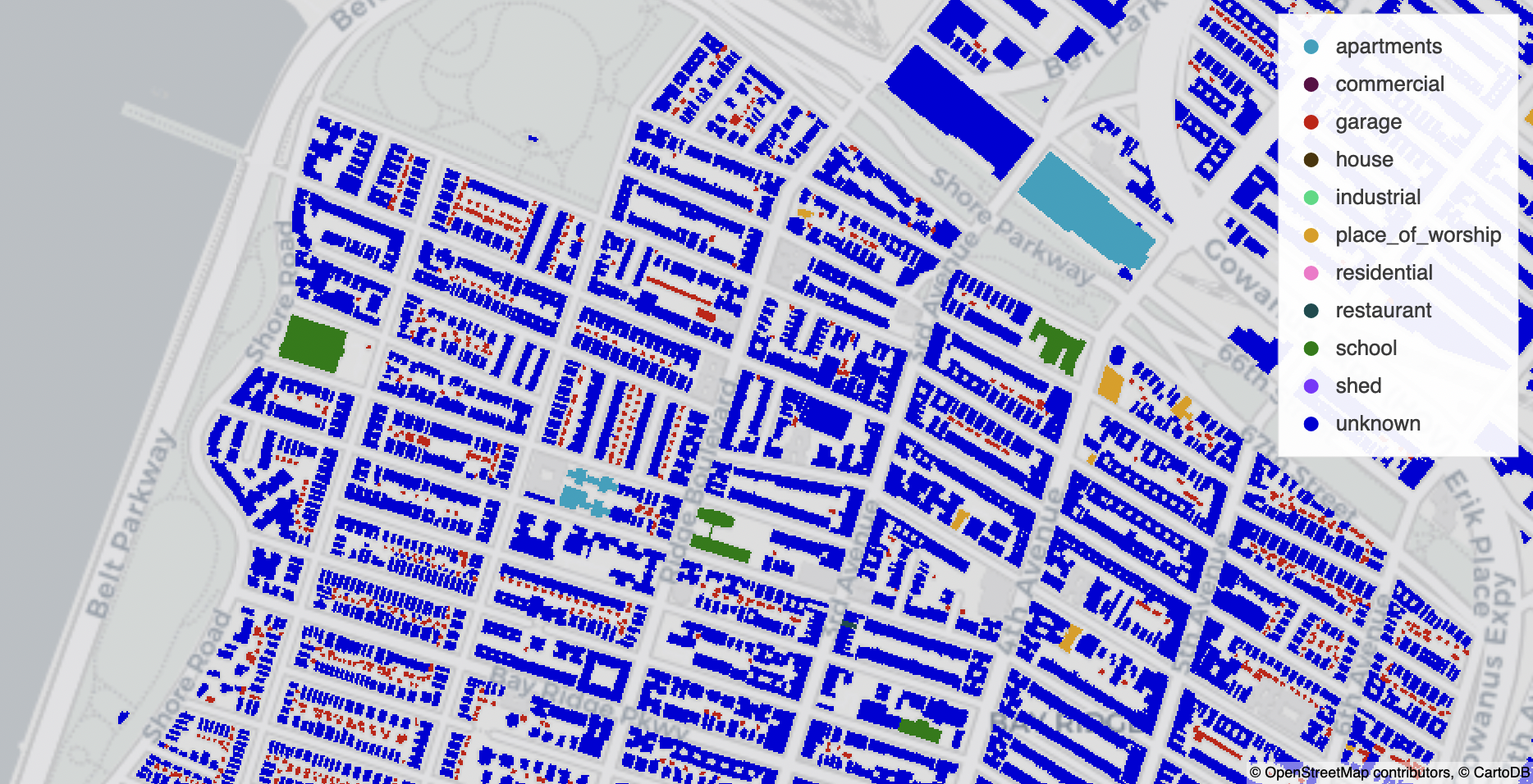
A larger example with polygons for the footprints of a million buildings in the New York City area can be run online at HoloViz examples.